Back to Resources

How Does WCM Simulate SMPS Magnetics with Finite Element Modeling?

Published by West Coast Magnetics, July 2026, based on our 2019 APEC presentation on finite element modeling of switch-mode power supply magnetics (available for download below); content reviewed and confirmed current as of publication.

West Coast Magnetics uses finite element modeling (FEM) in ANSYS Maxwell to simulate and validate SMPS transformer and inductor designs before building them. FEM divides a component into a mesh and solves the magnetic field in each element, and because SMPS windings are driven by square waves, WCM uses the transient (time-varying) solver rather than a sinusoidal one. Litz winding loss cannot be modeled directly in FEM, so WCM pairs it with LitzOpt, the Dartmouth Squared-Field-Derivative tool, and runs the heavy 3D cases on high-performance cloud computing.

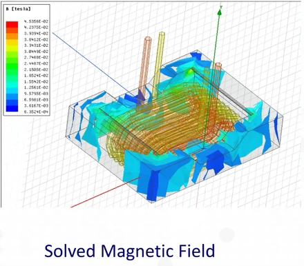
Solved magnetic flux density in a WCM SMPS transformer, computed in ANSYS Maxwell — A solved FEM result: the magnetic flux density (B, in tesla) through a WCM SMPS transformer, computed in ANSYS Maxwell. FEM produces the full field distribution, losses, and hot spots from the geometry and materials alone.

Finite element modeling (FEM) is a numerical method that divides a component into many small mesh elements (triangles in 2D, tetrahedra in 3D) and solves the governing field equations in each one, then assembles them into a full-field solution. For magnetics, ANSYS Maxwell uses FEM to solve Maxwell’s equations with a choice of solvers: magnetostatic (DC), eddy-current (sinusoidal), and transient (time-varying).

What FEM Does for a Magnetic Design

FEM lets a designer predict how a transformer or inductor will behave, its flux distribution, losses, and hot spots, from the geometry and materials alone, before any copper is wound. ANSYS Maxwell solves Maxwell’s equations across the mesh, in 2D or 3D, using the solver that matches the excitation: magnetostatic for DC, eddy-current for sinusoidal, and transient for time-varying waveforms.

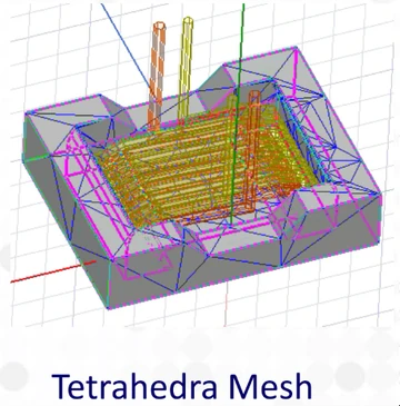
A 3D tetrahedral finite-element mesh over a WCM transformer model imported from SolidWorks — The tetrahedral mesh over a transformer model imported from SolidWorks. FEM accuracy depends on both the geometry fidelity and the mesh density, and finer meshes cost more computation.

The accuracy of the result depends directly on how faithful the geometry is and how fine the mesh is: a finer mesh resolves the field more accurately but costs more memory and time. That tradeoff is the central practical constraint of FEM, and managing it is part of doing the simulation well rather than just running it.

Why the Transient Solver for SMPS

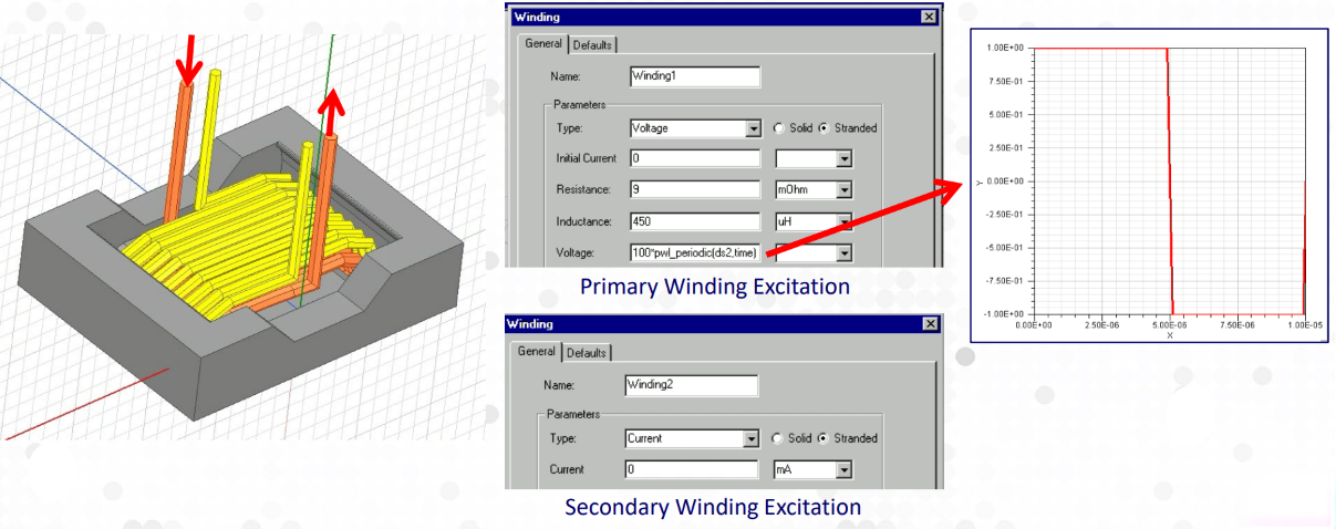
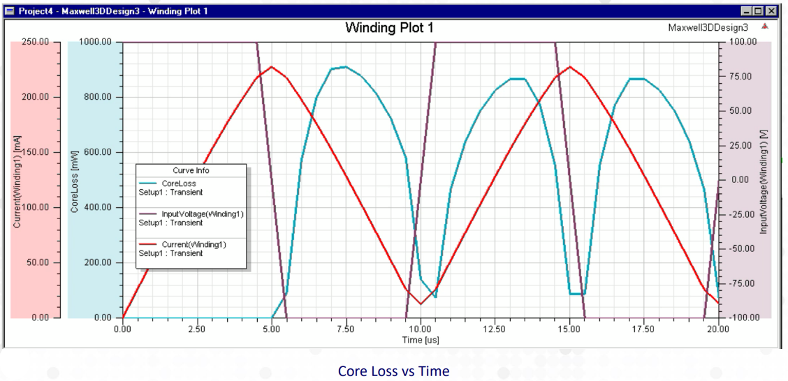
An SMPS transformer is not driven by a clean sine wave; it sees a square-wave voltage from the switching stage. A sinusoidal (eddy-current) solver cannot represent that correctly, so WCM uses the transient solver to simulate core loss under the actual square-wave excitation, for example a 100 V, 100 kHz square wave on the primary with the secondary open. Simulating the real waveform is what makes the predicted core loss trustworthy.

Defining winding excitation in ANSYS Maxwell: a square-wave voltage on the primary and an open secondary — Defining the excitation in ANSYS Maxwell: a square-wave voltage on the primary winding (with the resulting waveform) and an open secondary at 0 A, the setup for a transient core-loss simulation.

Transient simulation output: square-wave input voltage, winding current, and core loss versus time — The transient output: the square-wave input voltage, the resulting winding current, and the core loss over time. This is the waveform-accurate loss a sinusoidal solver cannot produce.

The Litz Problem: FEM Plus LitzOpt

FEM has a known limit with litz wire. It can model eddy-current losses in a solid conductor, but litz wire is bundles of thousands of fine strands, and meshing that geometry directly is impractical. At the same time, traditional modeling cannot estimate litz winding loss from manufacturer DC-resistance data alone, because that data does not capture the proximity effect.

WCM closes that gap by pairing FEM with LitzOpt, the litz-loss tool from Dartmouth’s Magnetic Component Research group. LitzOpt uses the Squared-Field-Derivative (SFD) method to compute per-strand loss from the rate of change of the field, which is exactly the part FEM cannot mesh economically. How litz is then specified from that analysis is covered in litz wire design for high-frequency windings, and how it fits the broader winding choice in foil vs litz vs wire.

Making 3D Practical: High-Performance Computing

A full 3D FEM simulation of an SMPS transformer is demanding on both memory and time. WCM runs those cases on high-performance cloud computing, using multiple cores and multithreading to overcome the memory and runtime limits that would otherwise force a coarser, less accurate model. That is what makes a high-fidelity 3D transient simulation a routine design tool rather than a special effort.

Why It Matters

Simulating a design in FEM before building it is how WCM turns a specification into a part that works the first time, rather than iterating physical prototypes to find the losses and hot spots. It is one input to WCM’s broader in-house development process, where competing designs are modeled, prototyped, and measured against the target. This capability was presented at APEC 2019 by WCM engineers Shuang Feng, Mary E. Clark, and Weyman Lundquist, and it remains part of how WCM designs. For the full design, build, and test capability set, see the WCM capabilities overview.

When standard components don’t fit your needs, our teams will engineer a solution.

FAQ

What is finite element modeling (FEM) for magnetics?

Finite element modeling is a numerical method that divides a component into many small mesh elements (triangles in 2D, tetrahedra in 3D), solves the governing field equations in each one, and assembles them into a full-field solution. For magnetics, ANSYS Maxwell uses FEM to solve Maxwell’s equations, letting a designer predict flux distribution, losses, and hot spots from the geometry and materials before building the part. It offers magnetostatic (DC), eddy-current (sinusoidal), and transient (time-varying) solvers in 2D and 3D.

Which ANSYS Maxwell solver does an SMPS transformer need?

The transient (time-varying) solver. An SMPS transformer is driven by a square-wave voltage from the switching stage, not a sine wave, so a sinusoidal eddy-current solver cannot represent it accurately. The transient solver simulates core loss under the real square-wave excitation, for example a 100 V, 100 kHz square wave on the primary with the secondary open, which is what makes the predicted loss trustworthy.

Why can’t FEM model litz wire loss directly?

Litz wire is made of thousands of fine, individually insulated strands, and meshing that geometry in FEM is impractical. FEM can model eddy-current losses in a solid conductor, but not an economical litz mesh. Traditional modeling from manufacturer DC-resistance data also fails, because it does not capture the proximity effect. WCM instead computes litz loss with LitzOpt and its Squared-Field-Derivative method.

What is LitzOpt and the Squared-Field-Derivative (SFD) method?

LitzOpt is a litz-wire winding-loss tool from Dartmouth’s Magnetic Component Research group. It uses the Squared-Field-Derivative (SFD) method, which calculates per-strand loss from the square of the rate of change of the magnetic field, to estimate and optimize litz winding loss, the part that FEM cannot mesh economically. WCM uses it alongside ANSYS Maxwell FEM.

Why does WCM use cloud computing for FEM?

A full 3D FEM simulation of an SMPS transformer is heavy on both memory and computation time. Running it on high-performance cloud computing, with multiple cores and multithreading, overcomes those limits so a high-fidelity 3D transient model is a practical routine tool rather than a compromise. Without it, a designer would be forced to a coarser mesh and a less accurate result.

Read the full presentation

How WCM Simulates SMPS Magnetics with FEM